
Abdul
Wasay
I take photonic chips from simulation to tape-out to measurement. Two years of PIC design, characterisation and lab automation at Fraunhofer HHI, and a master’s in theoretical physics on open quantum systems.
My work
Physicist who builds the tools as well as the chips
I grew up in Pakistan and came to Berlin for physics, where I completed both my bachelor’s and my master’s at TU Berlin with a grade of 1.3. Since 2024 I have worked in the Hybrid PICs group at Fraunhofer HHI, designing polymer and silicon nitride components, taking them to tape-out and measuring quantum light in the lab, while my master’s thesis took me deep into numerical methods for open quantum systems.
How I work
Outside the lab
- Music. I play piano and guitar.
- Reading. Novels from both Western and Japanese writers.
- Languages. I taught myself Japanese, far enough to follow conversations and read simple kanji.
- Long walks, the best place to think a problem through.
- Coffee. I worked as a barista, so cappuccino, latte, Milchkaffee or cortado: I make a serious cup.
Profile
Education and work
Grade 1.3. Thesis on second-order quantum state diffusion for non-Markovian open many-body lattice models.
Hybrid PICs group: design, simulation and characterisation.
Grade 1.3. Thesis on quantum trajectories for the local Redfield equation.
Tools I use today
Looking for PIC design, photonic characterisation and quantum engineering roles
Based in Berlin and eligible to work in Germany; open to roles anywhere in Germany or remote. Available from mid-November 2026.
The work in detail
Design simulations, lab data and live physics models, running in your browser. Jump to photonics, the lab or theory.
Photonic integrated circuits
I design passive components on polymer and silicon nitride platforms, from mode solving to GDSII mask. Every design I list here went into a fabrication run, and each one carries a tolerance analysis against realistic fabrication variance, using Ansys optiSLang and manual parameter sweeps to find optima that survive the fab.
Arrayed waveguide gratings
Four polymer AWG variants, 8 and 16 channels at 1550 nm, designed in both Lumerical and Luceda IPKISS. They separate SPDC photon pairs inside a PolyBoard system with −30 dB crosstalk.
MMI couplers and splitters
Five MMIs on silicon nitride (1×2, 1×3, 3×3, 4×4 and a 9×9 Talbot-effect splitter that distributes light for optical machine-learning training) and two on polymer.
785 nm PolyBoard chip
A full chip architecture in the visible range: fibre-to-chip interface, a thin-film-filter polarising beam splitter, tap coupler and MMI, with radial profiling to find the minimum bend radius of the polymer waveguides.
Thin-film filters
Geometric parametrisation across RGB, infrared and 1550 nm bands for polarising beam splitters, dichroic mirrors and bandpass filters.
Measured results
| Component | Platform | Result | Notes |
|---|---|---|---|
| 1×2 MMI | SiN | 98.2 % transmission | Split 48.8 % / 49.4 %, 1.8 % excess loss |
| 4×4 MMI | SiN | ≈4 % excess loss | Splitting uniform within 0.5 % |
| Spot-size converter | Polymer | up to 92 % coupling | Without 3D tapering, which the platform does not support |
| AWG in PolyBoard system | Polymer | −30 dB crosstalk | Measured in the photon-pair separation system |
9×9 Talbot-effect splitter, simulated field
Simulation- Platform
- Silicon nitride
- Model
- 3D FDTD, 1550 nm
- Simulated total
- —
- Port-to-port spread
- —
Schematic, not to scale: nine access waveguides on each side widen through linear tapers into the multimode section; the red port is the input in use.
3D FDTD at 1550 nm for two launch conditions. The central input is the design case and matches how the fabricated chip was measured; the edge input is the worst case. The red stub marks the input in use. Press Propagate light to watch the pattern build up from the input. Each run has a top-view field monitor, a cross-section monitor at the output tapers, and nine port monitors. Drag the field to pan, and zoom in to see the self-imaging pattern form. The device distributes light for optical machine-learning training.
16-channel polymer AWG from my IPKISS package
Simulation- Platform
- Polymer, fabricated
- Channels
- 16, 1526–1574 nm
- Channel spacing
- ≈3.2 nm
- Insertion loss
- 0.7–2.3 dB (simulated)
- Adjacent crosstalk
- below −70 dB (simulated)
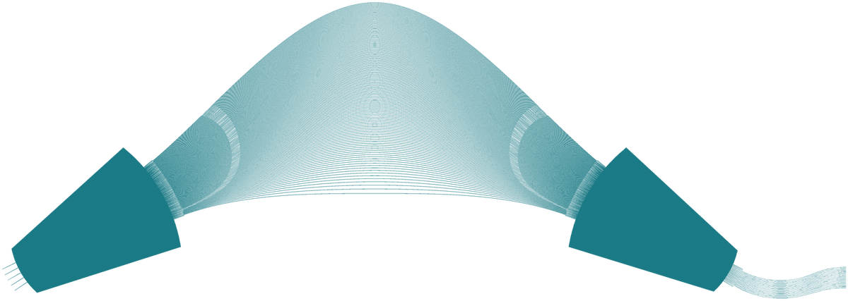
Mask layout of the AWG, shown without scale: light from the input spreads in the first star coupler, picks up a wavelength-dependent phase in the arrayed waveguides and refocuses onto one of the 16 outputs in the second star coupler.
Simulated transmission of all 16 channels. Drag the slider or the plot to tune. In pair mode a 775 nm pump splits into signal and idler photons whose energies add up to the pump photon (1/λs + 1/λi = 1/775 nm), so they sit on either side of 1550 nm and land in mirrored ports. That is how my AWGs split SPDC photon pairs. The test-laser mode shows what a single C-band probe would see.
MMI self-imaging explorerSet the port count and width, and watch the self-images formShow
MMI self-imaging explorer
InteractiveA symmetric input forms N equal images at L = 3Lπ/4N. The red line marks that plane, and the profile on the right is the light you would collect there. Assumes effective index 1.9 and λ = 1550 nm.
PolyBoard chip for BB84, block by blockThe design sweep behind each building block of the chipShow
PolyBoard chip for BB84, block by block
SimulationThe polymer chip architecture I designed for a quantum key distribution transmitter, simulated at 785 nm and 1550 nm. Pick a building block to see the sweep I used to choose its geometry; the marker shows the value that went into the layout.
Simulation sweeps (FDTD, EME and mode solver). Geometric parameters are shown relative to the value chosen for the layout.
PolyBoard PBS: thin-film-filter polarisation combinerThe polarising beam splitter of the PolyBoard chip, used to combine TE and TMShow
PolyBoard PBS: thin-film-filter polarisation combiner
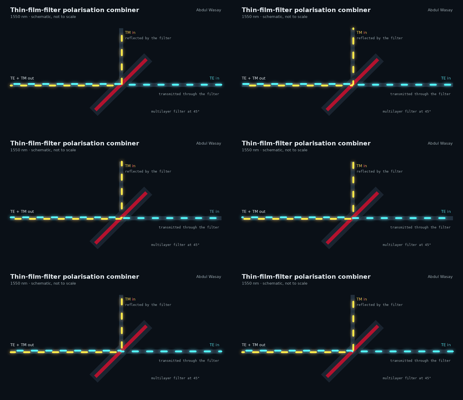
SimulationThe polarising beam splitter (PBS) of the PolyBoard chip, here used as a combiner. Two polymer waveguides carry TE and TM light into a multilayer dielectric filter set at 45° in a glue-filled trench. One polarisation passes through the filter, the other is reflected, and both leave through a shared output waveguide. I built the 3D FDTD model to analyse the combiner's dispersion across the band and to check how it tolerates fabrication errors; those tolerance results set the waveguide offsets around the filter in the fabricated device. Shown schematically; select a part to see its role.
- Filter angle
- 45°
- Purpose
- Dispersion, tolerances
- Function
- TE through, TM reflected
- Model
- 3D FDTD
Design automation: two AWG packages
Lumerical Python AWG PDK
Written from scratch: free propagation regions, array waveguides, design rules and the AWG calculation method, through simulation to GDSII mask generation.
Luceda IPKISS AWG package
A surrogate PDK with a custom material platform, built on IPKISS base functions. I added a router for arbitrary fixed-bend waveguides, because IPKISS only offered U- and S-bends.
- Minimum spacing between array waveguides
- Smooth taper between free propagation region and array
- Minimum resolvable feature size
- No waveguide crossings
- Minimum bend radius
- Automated N×N MMI optimisation with optiSLang and 3D FDTD, verified by EME, geometry read from the GDS layout (in progress, first stage live below)
- Single-mode and adiabatic taper simulations
- Mode coupling of Bragg reflection waveguides to pick the best fibre interface
- SPAD photon-production curves versus source angle in Lumerical FDTD
Robust N×N MMI optimiserThe fast first stage of the optimiser, running in your browserShow
Robust N×N MMI optimiser
In developmentThe fast first stage of my MMI optimisation pipeline, running live. A finite-difference solver finds every guided mode of the MMI, each access port is projected onto them, and the transfer matrix follows from mode propagation. A design is scored on its worst case over three wavelengths (1530, 1550, 1570 nm) and three fabrication width biases (−0.3, 0, +0.3 µm), with penalties for lithography limits and footprint.
Uses the placeholder indices from my code (generic polymer-like indices and core, TE), not platform material data. Length and pitch are scaled to the self-imaging theory for the current width, so the search space stays well conditioned when the width changes. The browser port reproduces the Python model to every printed digit. Stages 2–4 are written and so far tested against mock solvers. The optimiser is still in development and not yet on GitHub.
Quantum light in the lab
I characterise nonlinear photon-pair sources for quantum key distribution: periodically poled lithium niobate (PPLN) crystals and Bragg reflection waveguides (BRW). I measure phase-matching temperatures, wavelength tuning curves and SPDC pair peaks, and run the inverse process, second-harmonic generation, to check coupling and efficiency. The setup uses single-photon counters, a time tagger and a tunable diode laser, and I adapt it per project with custom splitters and pump-suppression filters.
BRW photon-pair source, from bare chip to sub-assembly
Illustrative dataOne chip followed from the bare waveguide into its packaged sub-assembly, measured at two temperatures. Pick a stage to see its pump-wavelength sweep and the time-tagger histograms behind it.
Illustrative data with the same structure as my measurements: 1-minute histograms per point, pairs counted in a 5 ns window around each setup’s coincidence peak and the accidental background subtracted. Packaging trades some pair rate for stability, and the sub-assembly keeps the coupling fixed between runs.
The measurement setupEvery component of the photon-pair setup, path by pathShow
The measurement setup
InteractiveThe fibre setup I built and run for photon-pair characterisation, shown in its general form; I adapt it for each chip or module. Select a path to follow it, or a component to see what it does.
Type-II PPLN photon-pair sourcePhase-matching sweeps, coincidence histograms and the CAR modelShow
Type-II PPLN photon-pair source
Illustrative data- Sweeps
- Pump wavelength, temperature
- Per point
- 1 min time-tagger histogram
- Pair window
- 2 ns, background-subtracted
- Figure of merit
- Net pairs and CAR
Illustrative data with the same structure as my measurements. Each point is a two-detector time-tagger histogram: pairs are counted in a 2 ns window around the coincidence peak and the accidental background, taken from the flat region beyond 60 ns, is subtracted; CAR is net pairs divided by accidentals in the same window. Pair generation switches on sharply above a threshold pump wavelength and falls off on the long-wavelength side, while the temperature acceptance is broad.
How CAR scales with pump powerA live model of coincidences versus accidentals as the pump power risesShow
How CAR scales with pump power
ModelPairs grow linearly with pump power, while accidental coincidences between unrelated photons grow quadratically, so CAR falls as you pump harder. The two curves are illustrative, one for a crystal source and one for a waveguide source; the histogram adds counting noise.
Choosing the fibre for a Bragg reflection waveguideMode overlap between the waveguide and lensed or standard fibresShow
Choosing the fibre for a Bragg reflection waveguide
SimulationThe BRW source is pumped at 775 nm in a Bragg mode that is wide and flat, so no round fibre mode matches it perfectly. I solved the mode of the etched ridge in Lumerical and computed its overlap with Gaussian fibre modes to decide which fibre to couple with. Here the overlap is recomputed live from the exported mode field, so you can also test misalignment.
Overlap η = |∫EBRW Efibre dA|² / (∫|EBRW|² dA ∫|Efibre|² dA) on the solver's non-uniform mesh, with a Gaussian fibre field exp(−r²/w₀²), w₀ = MFD/2. Dots are the mode solver’s own overlap results, which the live calculation reproduces. The optimum near 2.5 µm is why I couple this chip with a lensed fibre of 2.5 µm spot size rather than a cleaved fibre.
Aligning fibres with the photons themselves
Fibre-to-waveguide alignment usually relies on visible light. I built a signal chain that turns single-photon detector pulses into a steady voltage, so an automatic alignment tool can optimise coupling on the SPDC photons directly. It is the alignment loop in the setup diagram above.
- Python control of Thorlabs temperature controllers and a Toptica DLC pro tunable laser through the vendor SDKs
- Power stabilisation with a power regulator and wavelength sweeps through SweepMe!
- Reusable measurement scripts with live plotting, on-the-fly analysis and HDF5 storage
- Hanbury Brown–Twiss and coincidence measurements with time-tagged analysis on a qutools quTAG
- Chip coupling with fibre arrays, lensed fibres and cleaved fibres; cutback and wavelength-sweep loss measurements
- Cleanroom: ICP plasma-activated bonding of silicon wafers
Open quantum many-body dynamics
Real quantum systems leak into their environment, and that environment remembers. I developed a local expansion for second-order non-Markovian quantum state diffusion that avoids diagonalising the Hamiltonian. It gives a positivity-preserving unravelling, equivalent to the Redfield equation at second order, that scales to many-body lattices when combined with matrix product states.
Disordered XXZ spin chains with up to 35 sites, run as parallel stochastic trajectories on up to ≈52 GPUs of the TU Berlin mathematics cluster.
Correlated-noise generator for an Ohmic bathColoured-noise trajectories that drive the thesis methodShow
Correlated-noise generator for an Ohmic bath
Port of my Julia codeThe bath has spectral density J(ω) = γ ω e−ω/ωc at temperature T, so its correlation function α(t) = ∫ J(ω) [(n(ω)+1) e−iωt + n(ω) eiωt] dω is complex. The generator builds a kernel R(t) with α = R ⋆ R* from √S(ω), the square root of the FFT of α, and convolves it with complex white noise. Change the bath and the check reruns 2000 realisations in your browser.
Same parameters as my thesis script: γ = 0.06, time step 0.05, memory support of 5 time units before t = 0. In the thesis these trajectories drive the non-Markovian quantum state diffusion equation; the fine-grid noise is averaged onto the integrator's coarse time step with Simpson's rule and checked against the downsampled Toeplitz correlation matrix. Units are dimensionless with ℏ = kB = 1.
Code
Extended ITensors.jl with my own backend for the stochastic dissipator and the nonlinear stochastic differential equation solver, using MPS/MPO and TDVP. The noise generator and correlation calculator are fully self-written.
Verification
Convergence in the hard low-temperature regime, benchmarked against the Redfield equation. The physics studied: entanglement growth and energy transport.
Where it leads
Correlated, non-Markovian noise is what real qubits see. Next, I plan a public surface-code memory study under correlated noise with Stim and PyMatching, reusing this generator.